Computing the Mayer multiple

I've learnt about the Mayer mutliple from The Inverstor Podcast. The Mayer multiple is the ratio of the bitcoin price divided by the 200-day moving average. It is designed to understand the price of bitcoin without taking in account the short term volatility. It helps investors filter out their emotions during a bull run.

Let's see how to compute the Mayer mutliple in python.

First, we need to import the data, we will use Quandl to download data from coinbase

import quandl
btc_price_data = quandl.get("BCHARTS/COINBASEEUR")
btc_price_data.tail()

	Open	High	Low	Close	Volume (BTC)	Volume (Currency)	Weighted Price
Date
2018-12-12	2966.00	3076.71	2952.05	3026.00	1447.627465	4.372890e+06	3020.728514
2018-12-13	3025.19	3028.06	2861.15	2886.91	2125.242928	6.261750e+06	2946.369017
2018-12-14	2886.91	2919.00	2800.32	2835.50	2527.558347	7.256959e+06	2871.134083
2018-12-15	2835.49	2865.00	2781.47	2830.45	1267.004758	3.568614e+06	2816.575409
2018-12-16	2830.45	2830.45	2830.44	2830.45	0.144249	4.082886e+02	2830.447385

Next we need to compute the 200 days moving average of the price of bitcoin

moving_averages = btc_price_data[["Open" ,"High" ,"Low","Close"]].rolling(window=200).mean()
moving_averages.tail()

	Open	High	Low	Close
Date
2018-12-12	5507.88295	5611.72570	5380.60150	5491.43610
2018-12-13	5491.44155	5595.14440	5363.77840	5474.38560
2018-12-14	5474.39910	5577.89585	5347.27500	5457.99125
2018-12-15	5457.94930	5559.49145	5330.78235	5439.75570
2018-12-16	5439.71660	5540.89425	5313.62955	5422.17700

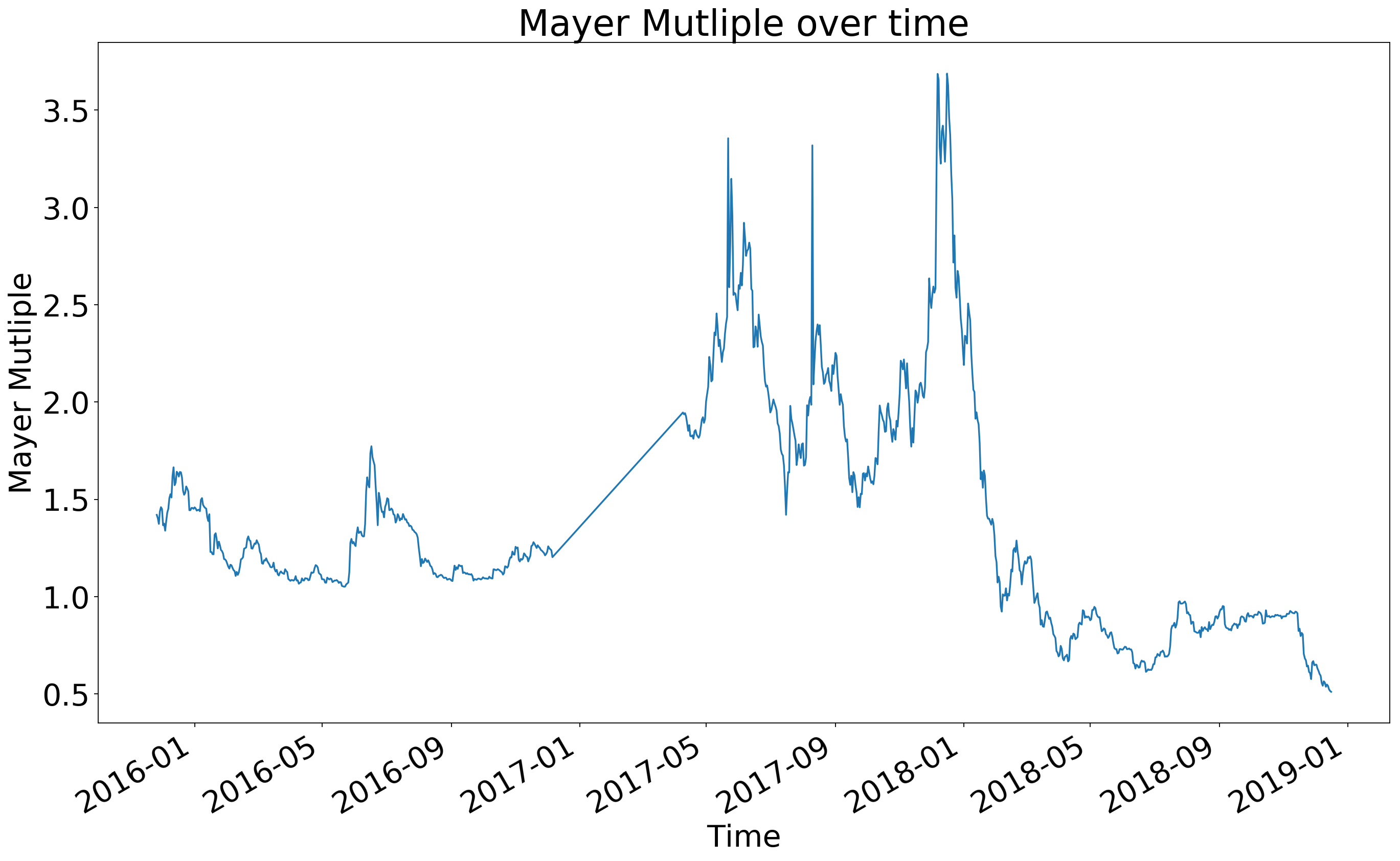
Finally, we can compute the ratio and plot it.

%matplotlib inline 
import matplotlib.pyplot as plt
plt.rcParams['savefig.dpi'] = 300
plt.rcParams['figure.dpi'] = 163
plt.rcParams['figure.autolayout'] = False
plt.rcParams['figure.figsize'] = 20, 12
plt.rcParams['font.size'] = 26


mayer_multiple = btc_price_data/moving_averages
mayer_multiple["High"].plot()
plt.title("Mayer Mutliple over time")
plt.ylabel("Mayer Mutliple")
plt.xlabel("Time")
print(f"Mayer multiple {mayer_multiple.iloc[-1]['High']}")
print(f"Mayer multiple average {mayer_multiple.mean()['High']}")

Mayer multiple 0.5108290958630005
Mayer multiple average 1.3789102045356179

png

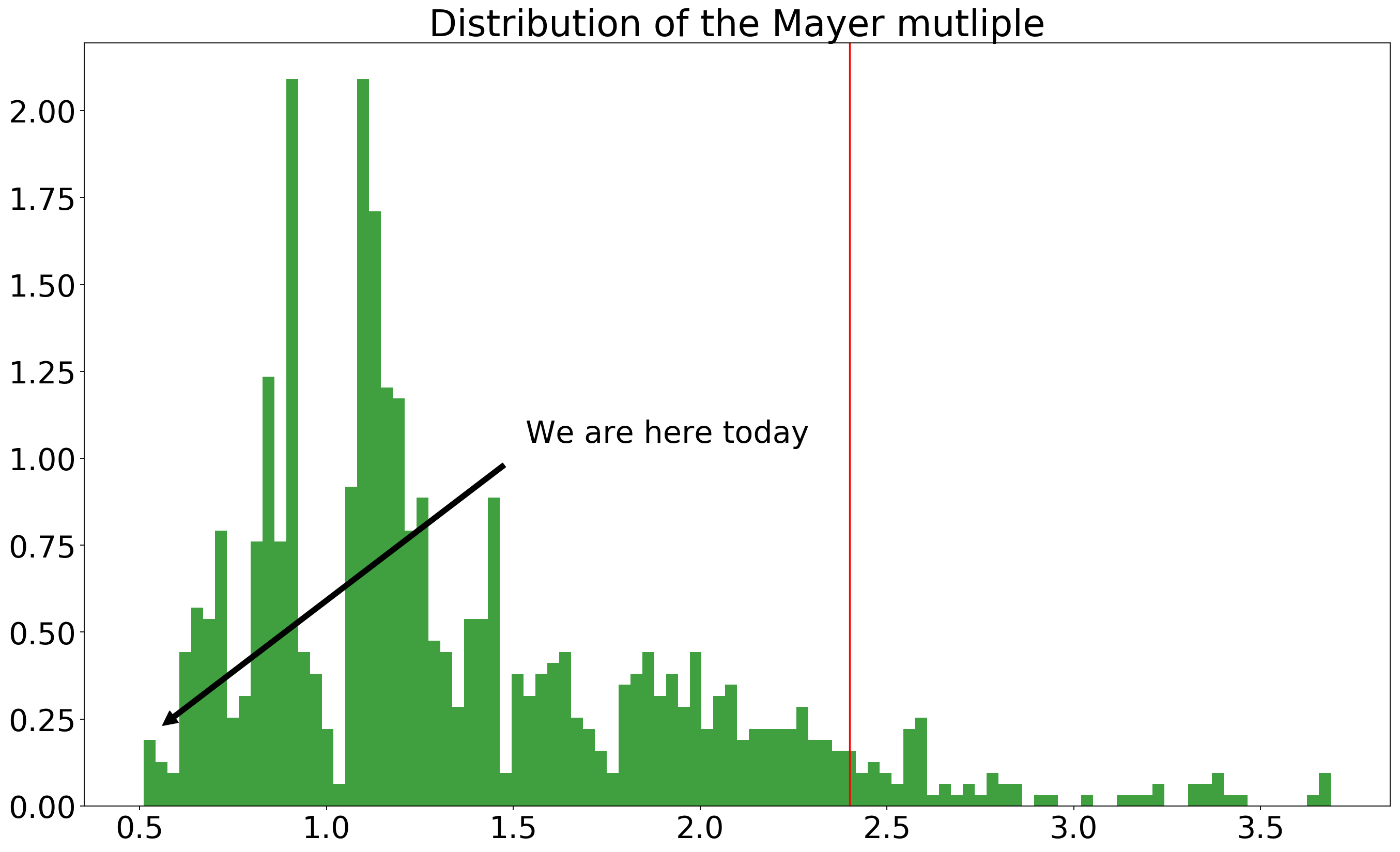
Lastly, I wanted to plot the distribution of the Mayer multiple

import numpy as np
x = mayer_multiple["High"].values
x = x[~np.isnan(x)]
n, a, patches = plt.hist(x, 100, facecolor='green', alpha=0.75, density=True)
plt.axvline(x=2.4, color="red")
plt.annotate('We are here today', 
             xy=(mayer_multiple.iloc[-1]["High"], 
                 n[(np.abs(bins-mayer_multiple.iloc[-1]["High"])).argmin()]), 
             xytext=(mayer_multiple.iloc[-1]["High"]*3,n.max()/2),
            arrowprops=dict(facecolor='black', shrink=0.05),
            )
plt.title("Distribution of the Mayer mutliple")
plt.plot()

[]

png